Vector Databases and RAG Systems — Building Intelligent LLM Applications
Complete guide to embeddings, retrieval-augmented generation, and semantic search
A Practical Guide to Building Knowledge-Enhanced AI Applications
1. Introduction to Vector Databases
What is a Vector Database?
A vector database is a specialized database designed to store and query high-dimensional vector embeddings efficiently. Unlike traditional databases that excel at exact matches (“find users named John”), vector databases excel at similarity searches (“find documents semantically similar to this query”).
Why This Matters: Vector databases are the backbone of modern AI applications—enabling semantic search, recommendation systems, and knowledge-augmented LLMs.
Key Characteristics:
- Similarity Search: Find the most similar items based on vector distance
- Scalability: Handle billions of vectors with sub-second query times
- AI-Native: Optimized for machine learning pipelines
Why LLMs Need Vector Databases
Large Language Models (GPT-4, Claude, Llama) have critical limitations that vector databases solve:
| LLM Limitation | Vector DB Solution |
|---|---|
| Knowledge Cutoff | Store and retrieve current information |
| Hallucinations | Ground responses in factual data |
| No Long-Term Memory | Persist context across sessions |
| Token Limits | Retrieve only relevant information |
| Lacks Domain Knowledge | Inject specialized expertise |
Real-World Applications
Vector databases power many AI applications you use daily:
- Customer Support Bots: Retrieve relevant help articles to answer user questions
- Enterprise Search: Find documents by meaning, not just keywords
- Code Assistants: Search codebases for similar implementations
- Research Tools: Find related papers and citations
- Recommendation Systems: “Users who liked X also liked Y”
- Chatbots with Memory: Remember past conversations
2. Understanding Embeddings
What are Embeddings?
Embeddings are numerical representations of data (text, images, etc.) as dense vectors of floating-point numbers. These vectors capture semantic meaning in a way machines can process and compare.
Example: The sentence “The quick brown fox” becomes a vector like:
[0.0123, -0.0456, 0.0789, -0.0234, 0.0567, ..., 0.0891] (1536 dimensions)How Embeddings Are Created
Neural networks (specifically transformers) create embeddings through a training process:
- Input Processing: Text is broken into tokens (words or subwords)
- Contextual Understanding: The transformer processes all tokens together, understanding relationships
- Vector Output: The final layer produces a fixed-size vector representing the entire input
Training Method - Contrastive Learning:
- The model sees pairs of similar texts (e.g., question and its answer)
- It learns to place similar texts close together in vector space
- Dissimilar texts are pushed apart
- After training on millions of pairs, the model understands semantic relationships
You don’t need to train your own embedding model. Pre-trained models like OpenAI’s text-embedding-3-small already understand language well. You just use them via API.
Why Similar Meanings Cluster Together
The training process creates a semantic space where:
- “Dog” and “Puppy” → Close together (similar meaning)
- “Dog” and “Airplane” → Far apart (unrelated)
- “King - Man + Woman ≈ Queen” → Vector arithmetic captures relationships
This is why searching for “automobile” can find documents about “cars”—they occupy nearby regions in the embedding space.
Semantic Space Visualization
When text is converted to embeddings, semantically similar items cluster together in vector space:
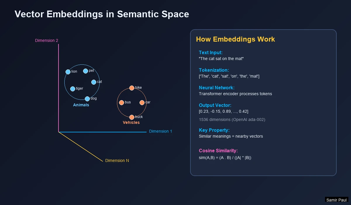
Key Insight: A query for “Kitten” naturally finds related animal terms, not fruits—because they’re close in vector space.
Dense vs Sparse Embeddings
| Type | Description | Example |
|---|---|---|
| Dense | Every dimension has a value; captures semantic meaning | [0.01, 0.74, 0.52, ...] |
| Sparse | Most dimensions are zero; captures keyword presence | {"cat": 4, "dog": 1} |
Modern systems combine both in hybrid search for semantic understanding AND keyword precision.
Dimension Trade-offs
More dimensions capture more nuance, but at a cost:
| Dimensions | Speed | Accuracy | Memory | Best For |
|---|---|---|---|---|
| 384 | Fastest | Good | ~1.5 KB/vector | Real-time apps, chatbots |
| 768 | Fast | Better | ~3 KB/vector | Balanced performance |
| 1536 | Medium | Excellent | ~6 KB/vector | Most production use cases |
| 3072 | Slower | Best | ~12 KB/vector | Maximum accuracy needed |
Rule of Thumb: Start with 1536 dimensions (OpenAI’s default). Only go larger if accuracy is critical and you have the infrastructure.
Popular Embedding Models
| Model | Dimensions | Provider | Best For |
|---|---|---|---|
text-embedding-3-small | 1536 | OpenAI | Cost-effective general use |
text-embedding-3-large | 3072 | OpenAI | Maximum accuracy |
all-MiniLM-L6-v2 | 384 | HuggingFace | Fast, open-source |
BGE-large-en-v1.5 | 1024 | BAAI | Top open-source performance |
embed-multilingual-v3.0 | 1024 | Cohere | 100+ languages |
3. Vector Search and Similarity
Distance Metrics
To find similar vectors, we measure “distance” between them:
Cosine Similarity (most common for text):
𝐬𝐢𝐦𝐢𝐥𝐚𝐫𝐢𝐭𝐲 = (𝐀 ⋅ 𝐁) ÷ (‖𝐀‖ ⨯ ‖𝐁‖)
- Score of 1.0 = Identical meaning
- Score of 0.0 = Completely unrelated
- Score of -1.0 = Opposite meaning
| Metric | Best For |
|---|---|
| Cosine | Text embeddings |
| Euclidean (L2) | Image embeddings |
| Dot Product | Normalized vectors |
Similarity Scoring Example
Query: “Is Windows 8 any good?”
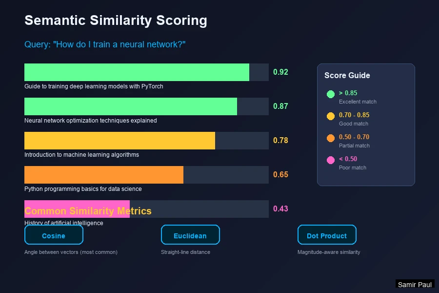
Pitfall: “Windows 10 is good” scores 0.88—as high as actual Windows 8 content! Embeddings treat version numbers as semantically similar. This is why hybrid search matters.
Vector Indexing Algorithms
Searching billions of vectors requires Approximate Nearest Neighbor (ANN) algorithms. Here’s how the main ones work:
HNSW (Hierarchical Navigable Small World)
The most popular algorithm for production systems. Think of it as a multi-level express train system:
How it works:
- Creates multiple layers of connected nodes (vectors)
- Top layer: Few nodes, long-distance connections (express trains)
- Bottom layer: All nodes, short-distance connections (local stops)
- Search: Start at top, quickly narrow down, then refine at bottom
Key Parameters:
M: Connections per node (higher = better recall, more memory)ef: Search width (higher = more accurate, slower)
Trade-off: Excellent speed and accuracy, but uses more memory than other methods.
IVF (Inverted File Index)
Uses clustering to organize vectors into buckets:
How it works:
- Training: Use k-means to create cluster centers (centroids)
- Indexing: Assign each vector to its nearest centroid
- Search: Find nearest centroids to query, then search only those clusters
Key Parameter:
nprobe: How many clusters to search (higher = more accurate, slower)
Trade-off: Fast for huge datasets, but requires training data and careful tuning.
PQ (Product Quantization)
Compression technique that shrinks vectors dramatically:
How it works:
- Split each vector into sub-vectors (e.g., 1536D → 8 chunks of 192D)
- Replace each sub-vector with a code pointing to a codebook entry
- Store only the codes (8 bytes instead of 6 KB!)
Trade-off: Massive memory savings (32-64x), but loses some accuracy.
Algorithm Comparison
| Algorithm | How It Works | Search Speed | Memory | Accuracy | Best For |
|---|---|---|---|---|---|
| HNSW | Graph navigation | O(log N) | High | Excellent | Production systems |
| IVF | Cluster search | O(√N) | Medium | Good | Large-scale search |
| PQ | Compressed codes | O(N) | Very Low | Moderate | Billions of vectors |
| IVF-PQ | Clusters + compression | O(√N) | Low | Good | Balance of all factors |
Most production systems use HNSW (Pinecone, Weaviate, Qdrant). It offers the best balance of speed and accuracy. Use IVF-PQ only when you have billions of vectors and limited memory.
4. RAG (Retrieval-Augmented Generation)
What is RAG?
RAG enhances LLM responses by retrieving relevant information from external sources before generating an answer.
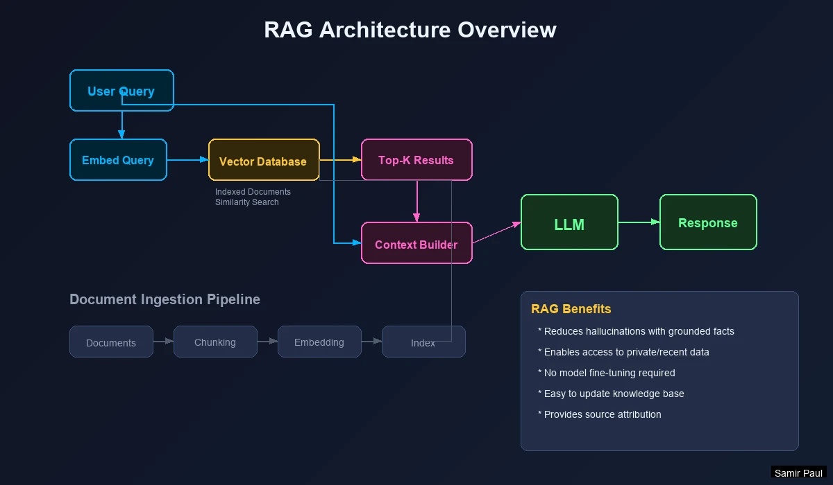
RAG Pipeline Steps
- User Query → User asks a question
- Query Embedding → Convert query to vector
- Vector Search → Find similar documents
- Context Retrieval → Fetch document content
- Prompt Construction → Combine query + context
- LLM Generation → Generate grounded answer
Why RAG Works: LLMs can’t read thousands of documents and remember them. Fine-tuning influences style, not knowledge. RAG retrieves relevant knowledge dynamically at runtime.
RAG Benefits
| Benefit | Description |
|---|---|
| No Retraining | Update knowledge by updating the database |
| Verifiable | Can cite sources for answers |
| Cost-Effective | Cheaper than fine-tuning |
| Up-to-Date | Add new information instantly |
Hallucination Prevention
RAG combats hallucinations by:
- Providing factual context in the prompt
- Instructing the LLM to answer only from provided context
- Allowing “I don’t know” when context is insufficient
5. Document Processing Pipeline
Basic Chunking Pipeline
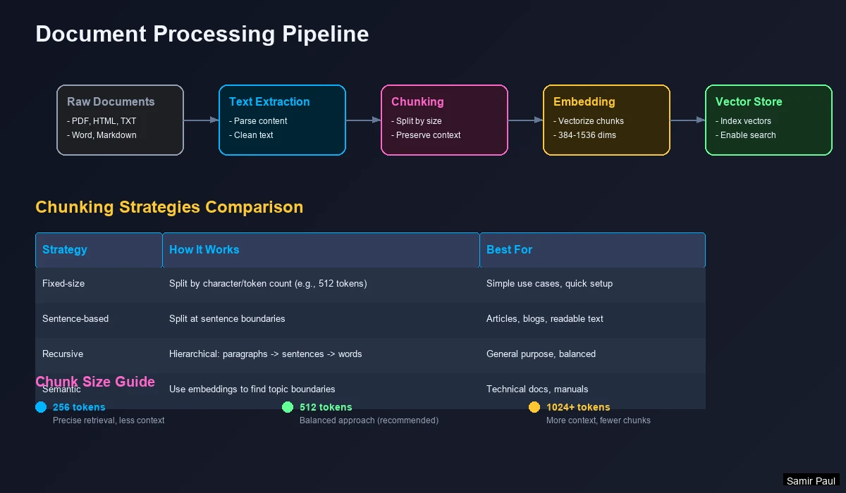
Steps:
- Extract raw text from documents (PDF, DOCX, HTML)
- Chunk into fixed-size pieces (500-1000 characters)
- Embed each chunk to a vector
- Store (vector, chunk) pairs in database
Chunking Strategies Compared
There are multiple ways to split documents. Each has trade-offs:
| Strategy | How It Works | Pros | Cons | Best For |
|---|---|---|---|---|
| Fixed-size | Split every N characters | Simple, predictable | May break mid-sentence | Quick prototyping |
| Sentence-based | Split at sentence boundaries | Grammatically correct | Variable chunk sizes | Articles, blogs |
| Recursive | Try paragraphs → sentences → words | Balances size and meaning | More complex | Mixed documents |
| Semantic | Use embeddings to find topic shifts | Best coherence | Computationally expensive | Technical docs |
Recursive Chunking (most recommended):
- First, try splitting by paragraph (
\n\n) - If chunks are still too large, split by sentence (
.) - If still too large, split by words
- This preserves natural document structure
Chunk Size Trade-offs
| Size | Tokens | Behavior | Best For |
|---|---|---|---|
| Small (~256) | ~64 | Precise retrieval, less context | Specific fact lookup |
| Medium (~512) | ~128 | Balanced approach | General Q&A |
| Large (~1024) | ~256 | More context, fewer chunks | Complex explanations |
| Very Large (~2048) | ~512 | Full paragraphs | Broad topic summaries |
Rule of Thumb: Match chunk size to expected query length. Short questions → smaller chunks. Complex questions → larger chunks.
Always use chunk overlap (10-20%). This prevents losing information that spans chunk boundaries. If a key fact is at the edge of two chunks, overlap ensures it appears in at least one complete chunk.
Advanced: Summarization Before Embedding
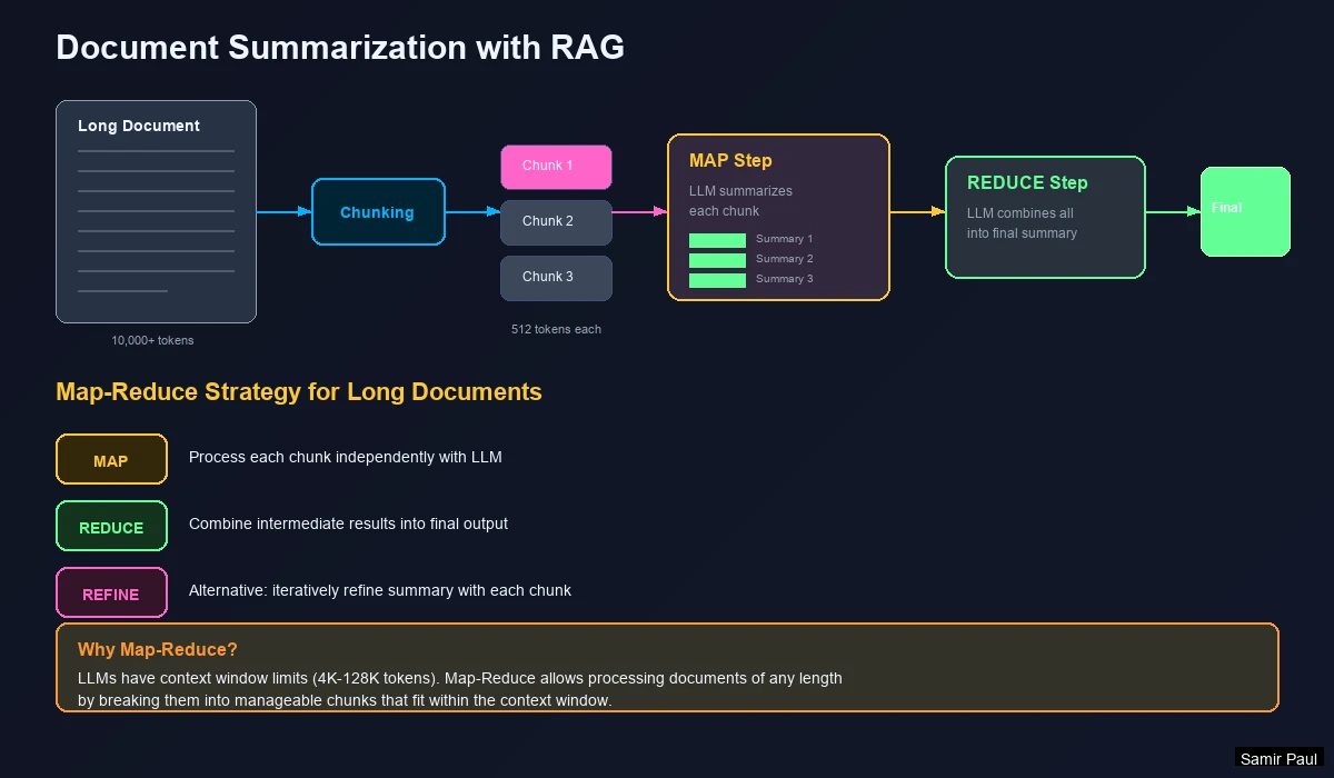
Benefits:
- Removes filler text that confuses embeddings
- Creates denser, more meaningful representations
- Normalizes formatting across document types
Parent Document Retrieval
For hierarchical documents (books, papers):
- Index smaller chunks (paragraphs) for precise retrieval
- When retrieved, also fetch the parent section for context
- Or use “windowed” approach—retrieve neighboring chunks
6. Prompt Engineering with RAG
Dynamic Few-Shot Prompting
Instead of hardcoding examples, retrieve relevant examples from a vector database:
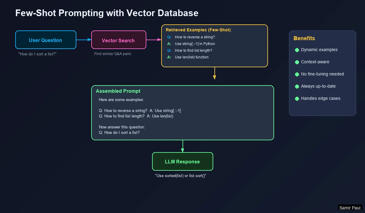
Flow:
- User asks a question
- Vector DB retrieves similar Q&A examples
- Examples are injected into the prompt
- LLM generates answer using those examples as guidance
Temperature Settings
| Temperature | Behavior | Best For |
|---|---|---|
| 0.0 - 0.3 | Deterministic, factual | RAG, Q&A, summarization |
| 0.4 - 0.7 | Balanced | General conversation |
| 0.8 - 1.0+ | Creative, diverse | Brainstorming, fiction |
For RAG: Use low temperature (0.0-0.3). Higher temperatures increase hallucination risk—defeating the purpose of retrieval-augmented generation.
7. Hybrid Search Strategies
Limitations of Pure Semantic Search
Semantic search can fail for:
- Entity-specific queries: “Windows 8” retrieves Windows 10/11 content
- Exact terminology: Medical terms, legal citations, product SKUs
- Negations: “not Python” still retrieves Python content
- Rare terms: Words not well-represented in training data
Understanding Keyword Search (Sparse)
Before combining approaches, understand how keyword search works:
TF-IDF (Term Frequency - Inverse Document Frequency)
A classic algorithm that scores documents based on keyword importance:
- TF (Term Frequency): How often does the word appear in this document?
- IDF (Inverse Document Frequency): How rare is this word across ALL documents?
- Score = TF × IDF
Intuition: If “quantum” appears 5 times in a document and is rare across your corpus, that document scores high for “quantum” queries.
BM25 (Best Match 25)
An improved version of TF-IDF used by most search engines:
- Adds document length normalization (short docs don’t unfairly win)
- Diminishing returns for repeated terms (10 mentions isn’t 10x better than 1)
- Tunable parameters (k1, b) for different use cases
When BM25 Shines: Exact terminology, product codes, legal citations, medical terms.
Combining Dense and Sparse Vectors
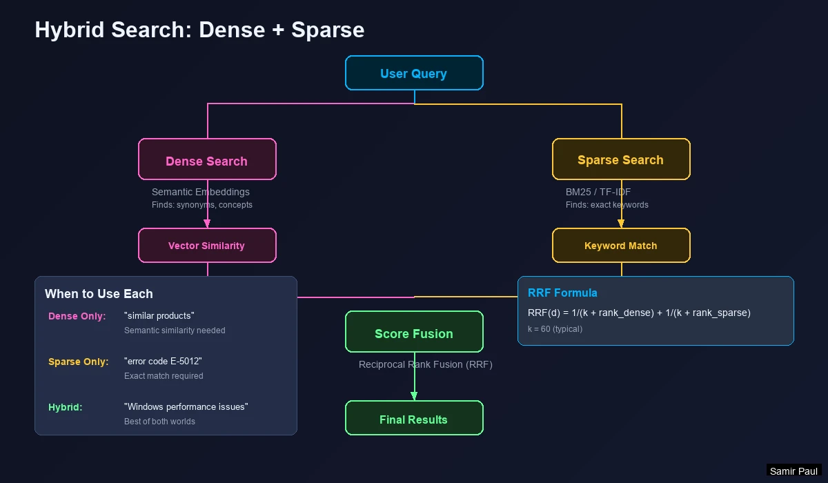
How It Works:
- Dense Vector → Captures semantic meaning (“car” finds “automobile”)
- Sparse Vector → Captures exact keywords (BM25/TF-IDF)
- Combined Query → Search both indexes simultaneously
- Score Fusion → Merge results using Reciprocal Rank Fusion (RRF)
Reciprocal Rank Fusion (RRF)
The standard method for combining search results:
𝐑𝐑𝐅(𝒅) = ∑ 𝟏 / (𝒌 + 𝐫𝐚𝐧𝐤ᵣ(𝒅)) for each 𝒓 ∈ 𝑹
Where:
d= documentR= set of ranking methods (dense, sparse)k= constant (typically 60)rank_r(d)= position of document d in ranking r
Why It Works: Documents appearing in BOTH dense and sparse results get boosted. A document ranked #3 in dense and #5 in sparse will outrank one that’s #1 in only one method.
When to Use Hybrid Search
| Scenario | Approach | Why |
|---|---|---|
| General Q&A | Dense (semantic) | Users phrase questions differently than docs |
| Technical docs | Hybrid | Need both concepts AND specific terms |
| Legal/Medical | Hybrid (favor sparse) | Exact terminology is critical |
| Product search with SKUs | Hybrid | Must match exact product codes |
| Conversational AI | Dense | Natural language varies widely |
Search Type Effectiveness
| Search Type | Finds | Misses | Example |
|---|---|---|---|
| Dense only | Synonyms, paraphrases | Exact codes, rare terms | “Tell me about vehicles” → finds “car”, “automobile” |
| Sparse only | Exact matches | Semantic variations | “SKU-12345” → finds exact match |
| Hybrid | Both semantic AND exact | Rarely misses anything | “Windows 8 issues” → finds Windows 8 specifically |
Rule of Thumb: If exact keywords matter, use hybrid search. Most modern vector databases (Pinecone, Qdrant, Weaviate) support it natively. Start with a 50/50 weight, then tune based on your data.
8. Reranking and Context Compression
Why Rerank?
Initial vector search isn’t perfect:
- Relevant documents may rank low
- Too much context overwhelms the LLM
- Documents buried in the middle get ignored (“lost in the middle” problem)
How Reranking Works
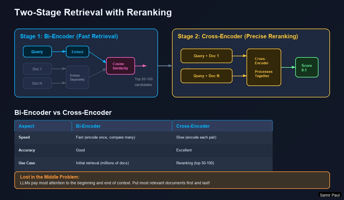
Two-Stage Retrieval:
- Stage 1: Vector search retrieves broad candidates (fast, ~100 docs)
- Stage 2: Reranker re-scores top candidates by relevance (precise, ~20 docs)
Bi-Encoder vs Cross-Encoder
The key to understanding reranking is understanding these two architectures:
Bi-Encoder (Used for Initial Retrieval)
- Embeds query and document separately
- Compares pre-computed embeddings using cosine similarity
- Speed: Can search millions of docs in milliseconds
- Accuracy: Good, but misses nuanced query-document relationships
Cross-Encoder (Used for Reranking)
- Processes query AND document together as one input
- Considers every word interaction between query and document
- Speed: Slow (must process each doc individually)
- Accuracy: Excellent (understands exact relevance)
| Type | How It Works | Speed | Accuracy | Stage |
|---|---|---|---|---|
| Bi-Encoder | Embed separately, compare | Milliseconds for millions | Good | Initial retrieval |
| Cross-Encoder | Process together | Seconds for dozens | Excellent | Reranking |
Analogy: Bi-encoders are like speed dating (quick impressions). Cross-encoders are like in-depth interviews (thorough evaluation).
Why Two Stages?
You can’t use cross-encoders for initial search—scoring 1 million documents would take hours. Instead:
- Stage 1 (Bi-Encoder): Cast a wide net, retrieve ~100 candidates fast
- Stage 2 (Cross-Encoder): Carefully evaluate top ~20 candidates
- Return the best ~5-10 to the LLM
This gives you the best of both worlds: speed AND accuracy.
Popular Reranking Models
| Model | Type | Speed | Accuracy | Notes |
|---|---|---|---|---|
rerank-english-v3.0 | Cohere API | Fast | Excellent | Production-ready, paid |
bge-reranker-large | Open Source | Medium | Excellent | Best open-source option |
ms-marco-MiniLM | Open Source | Fast | Good | Lightweight, fast |
cross-encoder/ms-marco-MiniLM-L-6-v2 | HuggingFace | Fast | Good | Easy to deploy |
Contextual Compression
Use a smaller LLM to:
- Extract only relevant portions from each document
- Discard irrelevant context
- Reduce token usage and cost
The “Lost in the Middle” Problem
Research shows LLMs have a U-shaped attention pattern:
- Pay most attention to the beginning of context
- Pay good attention to the end of context
- Ignore or forget information in the middle
Implications for RAG:
- Don’t just append retrieved docs in order of similarity score
- Put the MOST relevant document first
- Put the SECOND most relevant document last
- Less critical docs go in the middle
Lost in the Middle: If you retrieve 10 documents and the answer is in document #5, the LLM might miss it entirely. Reorder your context strategically!
9. Query Transformation Techniques
Sometimes the user’s query isn’t optimal for retrieval. Query transformation techniques improve retrieval by reformulating the query before searching.
HyDE (Hypothetical Document Embeddings)
Problem: User queries are short and may not match document vocabulary.
Solution: Generate a hypothetical answer, then search for documents similar to that answer.
How it works:
- User asks: “How do I fix memory leaks in Python?”
- LLM generates a hypothetical answer (even if imperfect)
- Embed the hypothetical answer (not the question)
- Search for real documents similar to this hypothetical
- Retrieved docs are often more relevant than direct query search
When to use: Technical queries, specialized domains where users and documents use different vocabulary.
Multi-Query Expansion
Problem: A single query may miss relevant documents phrased differently.
Solution: Generate multiple variations of the query and search with all of them.
How it works:
- Original query: “Python web frameworks”
- Generate variations:
- “Django vs Flask comparison”
- “Best backend frameworks for Python”
- “Building web apps with Python”
- Search with each query
- Combine results (using RRF or union)
When to use: Ambiguous queries, broad topics, when recall is more important than precision.
Step-Back Prompting
Problem: Specific questions may miss broader context needed to answer well.
Solution: Generate a more general version of the query first.
How it works:
- Specific query: “What’s the boiling point of water at 2000m altitude?”
- Step-back query: “How does altitude affect boiling point?”
- Retrieve documents for BOTH queries
- Combine context (general + specific)
When to use: Complex questions that require background knowledge.
Query Transformation Comparison
| Technique | When to Use | Latency Impact | Recall Improvement |
|---|---|---|---|
| HyDE | Technical/specialized queries | +1 LLM call | +15-25% |
| Multi-Query | Ambiguous queries | +3-5 searches | +10-20% |
| Step-Back | Complex questions | +1 LLM call, +1 search | Better context |
| Query Rewriting | Poor user queries | +1 LLM call | Variable |
Start simple: Most RAG systems work fine without query transformation. Add these techniques only if you see retrieval quality issues.
10. Advanced RAG Patterns
Basic RAG (chunk → embed → retrieve → generate) works well for simple use cases. For more complex scenarios, consider these advanced patterns:
CRAG (Corrective RAG)
Problem: Retrieved documents might be irrelevant or outdated.
Solution: Evaluate retrieval quality and self-correct if needed.
How it works:
- Retrieve documents normally
- Use an LLM to evaluate: “Are these documents relevant to the query?”
- If confident → proceed to generation
- If uncertain → try alternative retrieval (e.g., web search)
- If irrelevant → fall back to web search or “I don’t know”
When to use: Knowledge bases that may be incomplete, time-sensitive information.
Self-RAG (Self-Reflective RAG)
Problem: Not every query needs retrieval. Basic RAG always retrieves, wasting resources.
Solution: Let the LLM decide WHEN to retrieve and verify its own outputs.
How it works:
- LLM evaluates: “Do I need external information for this query?”
- If yes → retrieve and generate with context
- If no → generate directly from knowledge
- After generation → LLM verifies: “Is this answer supported by the context?”
When to use: Mixed query types (some factual, some conversational), cost-sensitive applications.
Agentic RAG
Problem: Complex questions require multiple retrieval steps and reasoning.
Solution: LLM acts as an agent that can retrieve, reason, and retrieve again.
How it works:
- LLM analyzes the question
- Breaks it into sub-questions if needed
- Retrieves information for each sub-question
- Reasons over retrieved information
- May retrieve again if gaps are found
- Synthesizes final answer
Example: “Compare the economic policies of the last 3 US presidents”
- Agent retrieves info on President 1
- Agent retrieves info on President 2
- Agent retrieves info on President 3
- Agent synthesizes comparison
When to use: Research questions, multi-hop reasoning, complex analysis.
RAG Pattern Selection
| Pattern | Complexity | Best For | Key Benefit |
|---|---|---|---|
| Basic RAG | Simple | Straightforward Q&A | Easy to implement |
| CRAG | Medium | Incomplete knowledge bases | Handles retrieval failures |
| Self-RAG | Medium | Mixed query types | Efficient (skips unnecessary retrieval) |
| Agentic RAG | High | Complex research | Multi-step reasoning |
Start with Basic RAG. Only add complexity when you have evidence that basic RAG isn’t working. Each additional pattern adds latency and cost.
11. RAG Evaluation Framework
You can’t improve what you don’t measure. RAG systems require evaluation at two stages: retrieval and generation.
Retrieval Metrics
These measure how well your system finds relevant documents:
| Metric | What It Measures | Formula | Good Score |
|---|---|---|---|
| Recall@k | % of relevant docs in top k results | relevant_in_k / total_relevant | > 0.8 |
| Precision@k | % of top k results that are relevant | relevant_in_k / k | > 0.6 |
| MRR | Position of first relevant result | 1 / rank_of_first_relevant | > 0.7 |
| NDCG | Ranking quality (position matters) | DCG / ideal_DCG | > 0.7 |
Example: For query “What is RAG?”, if you retrieve 10 docs and 3 are relevant:
- If relevant docs are at positions 1, 2, 5 → Good (high MRR, good NDCG)
- If relevant docs are at positions 6, 8, 10 → Bad (low MRR, poor NDCG)
Generation Metrics (RAGAS Framework)
RAGAS is the standard framework for evaluating RAG generation quality:
| Metric | What It Measures | How It’s Calculated |
|---|---|---|
| Faithfulness | Is answer grounded in context? | LLM checks if claims are supported |
| Answer Relevancy | Does answer address the question? | LLM scores relevance |
| Context Precision | Are retrieved docs actually useful? | % of context that contributed to answer |
| Context Recall | Did we retrieve all needed info? | Can answer be derived from context alone? |
Building an Evaluation Dataset
To evaluate your RAG system, you need:
- Test Questions: 50-100 representative queries
- Ground Truth Answers: What the correct answer should be
- Relevant Documents: Which docs should be retrieved
Quick Start:
- Extract real user questions from logs
- Have domain experts write answers
- Run evaluation weekly to catch regressions
Evaluation Best Practices
- Separate retrieval and generation evaluation - A bad answer might be due to poor retrieval OR poor generation
- Test edge cases - Queries with no answer, ambiguous queries, multi-hop questions
- Track metrics over time - Catch regressions early
- Use human evaluation for final quality assessment - Automated metrics don’t catch everything
Minimum viable evaluation: Start with 50 test questions and track Recall@10 for retrieval and Faithfulness for generation. Expand from there.
12. Debugging RAG Failures
When your RAG system gives wrong answers, use this systematic approach to find and fix the problem.
Common Failure Modes
| Symptom | Likely Cause | Solution |
|---|---|---|
| Returns irrelevant documents | Embedding model mismatch | Try domain-specific embeddings |
| Misses obvious answers | Chunks too small | Increase chunk size + overlap |
| “I don’t know” for known facts | Document not indexed | Check ingestion pipeline |
| Contradictory answers | Multiple conflicting sources | Add source reliability scoring |
| Slow responses | Too many docs retrieved | Reduce k, add reranking |
| Hallucinations despite context | LLM ignoring context | Lower temperature, stronger instructions |
| Wrong version info | Semantic similarity ignores numbers | Use hybrid search |
Debugging Checklist
When a query fails, check these in order:
1. Is the document even in the index?
- Search for an exact phrase from the expected document
- If not found → ingestion problem
2. Is the document retrieved?
- Look at similarity scores of retrieved docs
- If expected doc has low score → embedding or chunking problem
3. Is the right chunk retrieved?
- Check if the answer spans multiple chunks
- If answer is split → adjust chunk size/overlap
4. Is the LLM using the context?
- Check if answer matches retrieved context
- If LLM ignores context → adjust prompt, lower temperature
5. Is there conflicting information?
- Check for contradictory docs in results
- If present → add source filtering or recency scoring
Retrieval Quality Debugging
Test #1: Direct phrase search
- Search for exact text from a document you know exists
- If it doesn’t appear in top 10 → indexing problem
Test #2: Synonym search
- Search using synonyms of known document content
- If it works → your embedding model is fine
- If it fails → consider different embedding model
Test #3: Compare dense vs sparse
- Run query through dense search only
- Run query through sparse (keyword) search only
- Compare results → decide if hybrid search would help
When to Suspect Each Component
| Component | Suspect If… |
|---|---|
| Chunking | Answers are partially correct, missing context |
| Embedding Model | Synonyms don’t match, domain terms fail |
| Index Config | High recall but slow, or fast but missing results |
| Retrieval k | Good docs exist but not in top k |
| Reranking | Good docs retrieved but ranked low |
| Prompt | Correct context but wrong answer |
| LLM Temperature | Answers vary wildly, or include made-up facts |
Don’t guess - measure! Log every query, retrieval result, and answer. Use these logs to identify patterns in failures.
13. Cost Optimization
RAG systems can get expensive at scale. Here’s how to optimize costs without sacrificing quality.
Cost Components
| Component | Cost Driver | Typical Cost |
|---|---|---|
| Embedding API | Per token | ~$0.02 per 1M tokens |
| Vector Database | Storage + queries | $0.01-0.10 per 1K queries |
| LLM API | Input + output tokens | $0.50-5.00 per 1K queries |
| Reranking | Per document scored | ~$0.001 per document |
Key Insight: LLM calls dominate costs (often 80-90% of total).
Cost Reduction Strategies
1. Query Routing (Biggest Impact)
Not every query needs RAG. Route simple queries directly to the LLM.
- “What’s 2+2?” → Direct LLM (no retrieval needed)
- “What’s our refund policy?” → RAG (needs company docs)
Savings: 30-50% reduction in RAG operations.
2. Aggressive Caching
Cache at multiple levels:
- Query cache: Same query → same results
- Embedding cache: Same text → same embedding
- Answer cache: Frequent questions → cached answers
Savings: 20-40% reduction in API calls.
3. Tiered Retrieval
Only use expensive operations when needed:
- Fast vector search (always)
- Reranking (only if initial results are uncertain)
- Query transformation (only if initial retrieval fails)
Savings: 15-25% reduction in compute.
4. Context Optimization
Reduce tokens sent to LLM:
- Retrieve fewer documents (5 instead of 10)
- Use smaller chunks
- Compress context before sending
Savings: 20-40% reduction in LLM costs.
5. Model Selection
Use cheaper models for appropriate tasks:
| Task | Expensive Option | Cheaper Alternative |
|---|---|---|
| Embedding | text-embedding-3-large | text-embedding-3-small |
| Query routing | GPT-4 | GPT-3.5 or classifier |
| Simple Q&A | GPT-4 | GPT-3.5 or Claude Haiku |
| Complex reasoning | GPT-4 | Keep GPT-4 (worth the cost) |
Cost Estimation Example
Scenario: 10,000 queries/month, 5 docs retrieved per query
| Approach | Embedding | Vector DB | LLM | Total/Month |
|---|---|---|---|---|
| Basic RAG | $0.20 | $1.00 | $50.00 | ~$51 |
| With reranking | $0.20 | $1.00 | $70.00 | ~$71 |
| Optimized | $0.10 | $0.50 | $25.00 | ~$26 |
Optimizations applied: Query routing (50%), caching (20%), context compression (30%).
Measure before optimizing. Log costs per query type. You’ll often find 80% of costs come from 20% of query types—focus there first.
14. Popular Vector Databases
| Database | Type | Key Features | Best For |
|---|---|---|---|
| Pinecone | Managed SaaS | Serverless, hybrid search, easy setup | Production without DevOps |
| Weaviate | Open Source/Cloud | GraphQL API, built-in ML modules | Flexible deployments |
| Qdrant | Open Source/Cloud | Rust-based, very fast, good filtering | High performance needs |
| Milvus | Open Source | Distributed, GPU support, massive scale | Billions of vectors |
| Chroma | Open Source | Simple API, in-memory option | Prototyping, local dev |
| pgvector | Postgres Extension | SQL integration, familiar tooling | Teams using Postgres |
Deployment Options
| Option | Pros | Cons | Best For |
|---|---|---|---|
| Managed SaaS (Pinecone) | Zero DevOps, high reliability | Higher cost, vendor lock-in | Small teams, quick start |
| Managed Cloud (Weaviate Cloud, Qdrant Cloud) | Balance of control and convenience | Medium cost | Growing teams |
| Self-Hosted (Milvus, Qdrant, Weaviate) | Full control, lowest cost at scale | DevOps required | Large teams, enterprises |
Choosing a Vector Database
Choose Pinecone if: You want zero infrastructure management and fastest time-to-production.
Choose Weaviate if: You need flexibility and like GraphQL APIs.
Choose Qdrant if: Performance is critical and you want both cloud and self-hosted options.
Choose Milvus if: You have billions of vectors and need distributed architecture.
Choose Chroma if: You’re prototyping or building local-first applications.
Choose pgvector if: You already use PostgreSQL and want to add vector search without new infrastructure.
Production Considerations
Security
- Never expose API keys in client-side code
- Implement rate limiting
- Sanitize queries to prevent prompt injection
- Use row-level security for multi-tenant applications
Performance:
- Batch embedding requests when indexing
- Use async operations for concurrent retrieval
- Cache frequently-asked queries
- Monitor query latency and adjust index parameters
Reliability:
- Set up automated backups
- Use replicas for high availability
- Implement graceful degradation when DB is slow
15. Best Practices Summary
Chunking Checklist
- Preserve context: Don’t split mid-sentence
- Use overlap: 10-20% prevents information loss
- Respect structure: Use headers as natural break points
- Include metadata: Store source, page number, section title
- Test empirically: Evaluate with different chunk sizes
Embedding Model Selection
| Use Case | Model | Rationale |
|---|---|---|
| General English | text-embedding-3-small | Cost-effective |
| Maximum accuracy | text-embedding-3-large | Best quality |
| Multi-language | embed-multilingual-v3.0 | 100+ languages |
| Open-source | BGE-large-en-v1.5 | Top OSS performance |
| Low latency | all-MiniLM-L6-v2 | Fast, 384 dimensions |
Key Takeaways
- Embeddings transform text into searchable vectors capturing semantic meaning
- Vector databases enable fast similarity search at scale (HNSW is the standard)
- RAG grounds LLM responses in factual, retrievable knowledge
- Chunking significantly impacts quality—use recursive chunking with overlap
- Hybrid search combines semantic + keyword for best coverage
- Reranking improves precision using cross-encoders
- Evaluation is essential—track Recall@k and Faithfulness at minimum
- Cost optimization starts with query routing and caching
Implementation Roadmap
Phase 1: Basic RAG (Start here)
- Choose embedding model (start with
text-embedding-3-small) - Set up vector database (Pinecone for managed, Chroma for local)
- Implement basic chunking (512 tokens, 10% overlap)
- Build retrieve → generate pipeline
- Test with 20-30 sample questions
Phase 2: Quality Improvements (When basic RAG isn’t enough)
- Add hybrid search if keyword matching matters
- Add reranking if relevant docs are retrieved but ranked low
- Adjust chunk sizes based on retrieval quality
- Build evaluation dataset, track metrics
Phase 3: Advanced Features (For complex use cases)
- Query transformation (HyDE, multi-query) for better retrieval
- CRAG/Self-RAG for handling failures
- Agentic RAG for multi-hop reasoning
- Cost optimization for scale
Start Simple, Iterate
Don’t add complexity until you have evidence it’s needed. Each additional component adds latency, cost, and maintenance burden.
The best RAG system is the simplest one that meets your quality requirements.
Quick Decision Guide
| Question | If Yes → | If No → |
|---|---|---|
| Do exact keywords matter? | Use hybrid search | Dense search is fine |
| Are relevant docs ranked low? | Add reranking | Skip reranking |
| Do queries use different vocabulary than docs? | Try HyDE | Basic retrieval is fine |
| Are some queries too complex? | Consider Agentic RAG | Basic RAG is fine |
| Is cost a concern? | Implement query routing + caching | Optimize later |
Further Reading: